Machine Learning

Gekko specializes in optimization, dynamic simulation, and control. The ML module in GEKKO interfaces compatible machine learning algorithms into the optimization suite to be used for data-based optimization. Trained models from scikit-learn, gpflow, nonconformist, and tensorflow are imported into Gekko for design optimization, model predictive control, and physics-informed hybrid modeling.

Machine Learning Interface models

These functions allows interfaces of various models into Gekko. They can be found in the ML subpackage of gekko, imported like so:

from gekko import ML

Model = ML.Gekko_GPR(model,Gekko_Model,modelType='sklearn',fixedKernel=True)

Convert a gaussian process model from sklearn into the Gekko package.

model: The first argument is the trained gaussian model, either from sklearn GaussianProcessRegressor or a model from gpflow. Custom kernels are not implemented, but all kernels and combinations of kernel in sklearn are allowed.

Gekko_Model: Gekko model (created by GEKKO()) that is appended with the new GPR model.

modeltype: sklearn indicates that the model is from scikit-learn, otherwise from gpflow. If it is not sklearn, it convert from gpflow to sklearn.

fixedKernel: conversion from gpflow to sklearn. If it is set to True, the kernel hyperparameters are set to fixed; otherwise, False allows the hyperparameters to be changed during training.

Model = ML.Gekko_SVR(model,Gekko_Model)

Imports an SVR model into Gekko.

model: Model must be a variant of sklearn svm.SVR() or svm.NuSVR().

Gekko_Model: Gekko model (created by GEKKO()) that is appended with the new SVR model.

Model = ML.Gekko_NN_SKlearn(model,minMaxArray,Gekko_Model)

Import an sklearn Neural Network into Gekko.

model: model trained with the MLPRegressor function from sklearn.

minMaxArray: min-max array for scaling created by the custom min max scaler. This is necessary as neural networks often use a scaled dataset.

Gekko_Model: Gekko model (created by GEKKO()) that is appended with the new NN model.

Model = ML.Gekko_LinearRegression(model,Xtrain,RMSE,Gekko_Model)

Import a trained linear regression model from sklearn. This model calculates uncertainty through the delta method for regression methods.

model: trained model from sklearn as a Ridge Regression or Linear Regression model.

Xtrain: input training set, needed to calculate the prediction interval.

RMSE: root mean squared error calculated during training for the entire data set. This is used to calculate the prediction interval.

Gekko_Model: Gekko model (created by GEKKO()) that is appended with the new Linear Regression model.

Model = ML.Gekko_NN_TF(model,minMaxArray,Gekko_Model,n_output=2,activationFxn)

Import a Tensorflow and Keras Neural Network into Gekko. A specific loss function must be used during training to calculate uncertainty.

model: trained model from the TensorFlow.

minMaxArray: min-max array for scaling created by the custom min max scaler. This is necessary as neural networks often use a scaled dataset.

Gekko_Model: Gekko model (created by GEKKO()) that is appended with the new Neural Network model.

output: output dimensions; 1=prediction only, 2=predictions and uncertainty through a loss function.

activationFxn: activation function used between layers.

Model = ML.Boootstrap(models,Gekko_Model)

Perform an ensemble/bootstrap calculation method.

models: an array of models including GPR, SVR, and/or sklearn-NN models.

Gekko_Model: Gekko model (created by GEKKO()) that is appended with the new Ensemble model.

Model = ML.Conformist(modelinfo,Gekko_Model)

Conformal prediction wrapper for the previous listed machine learning models.

modelinfo: a 2-length array; the first item is the model (one of the above ones), and the second is a constant margin used for prediction intervals; it can be calulculated through conformal prediction methods.

Gekko_Model: Gekko model (created by GEKKO()) that is appended with the new conformal prediction method.

Model = ML.Delta(modelinfo,Gekko_Model)

Delta uncertainty wrapper for previous listed machine learning models.

modelinfo: a 3-length array; the first item is the model, the second is the RMSE from training, and the third is the x component of the training set.

Gekko_Model: Gekko model (created by GEKKO()) that is appended with the new conformal prediction method.

Model = ML.ScalerWrapper(model,Scaler,m)

Scaler wrapper for the models previously listed (unnecesary for neural networks); based on the custom Gekko min max scaler, it scales the input and unscales the output for model usage and prediction.

model: Machine learned model.

Scaler: custom scaler with data.

Gekko_Model: Gekko model (created by GEKKO()) that is appended with the new Scaler wrapper.

prediction = Model.predict(xi,return_std=True):

For any model class built by the above functions, the function predict is called to generate a prediction.

xi: input array. It must be the same shape as the features used to train the model. It can be scalar/array quantities, or it can be gekko variables as the input can be gekko variables. It allows optimization and control to be accessible to these models.

return_std: return standard deviation of prediction. For most models, this return 0 as this is not natively calculated. If the model is a gaussian model or is wrapped in one of the wrappers, then it provides an uncertainty. Some methods may increase runtime of the process, especially if the training set is large for the model.

Scaler = ML.CustomMinMaxGekkoScaler(data,features,label)

This scaler wraps around a dataset and scales it for use of neural networks or models wrapped in the scaler wrapper. It provides the same functionality as the min-max scaler in scikit-learn, except it is performed with Gekko variables.

Example problem

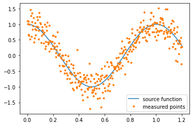
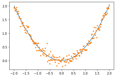
The example problem is a simple case study for the integration of Machine Learning models into Gekko. Noise is added to the data to represent measurement uncertainty and create a necessity for fitting a regression model to the data.

import numpy as np
import matplotlib.pyplot as plt

#Source function to generate data
def f(x):
    return np.cos(2*np.pi*x)

#represent noise from a data sample
N = 350
xl = np.linspace(0,1.2,N)
noise = np.random.normal(0,.3,N)
y_measured = f(xl) + noise

plt.plot(xl,f(xl),label='source function')
plt.plot(xl,y_measured,'.',label='measured points')
plt.legend()
plt.show()

Gekko’s optimization functionality is used to find a minimum of this function.

from gekko import GEKKO
m = GEKKO()
x = m.Var(0,lb=0,ub=1)
y = m.Intermediate(m.cos(x*2*np.pi)) #function is used here
m.Obj(y)
m.solve(disp=False)
print('solution:',y.value[0])
print('x:',x.value[0])
print('Gekko Solve Time:',m.options.SOLVETIME,'s')

solution: -1.0
x: 0.5
Gekko Solve Time: 0.0078999999996 s

If the original source function is unknown, but the data is available, data can be used to train machine learning models and then these trained models can be used to optimize the required function. In this case, the models are being used as the objective function, but they can be used as constraint functions as well. Currently, Gaussian Process Regression, Support Vector Machines, and Artificial Neural Networks from sklearn can be interfaced and integrated into Gekko. Below is a basic training script for each of the three models.

#Import the ML interface functions
from gekko.ML import Gekko_GPR,Gekko_SVR,Gekko_NN_SKlearn
from gekko.ML import Gekko_NN_TF,Gekko_LinearRegression
from gekko.ML import Bootstrap,Conformist,CustomMinMaxGekkoScaler
import pandas as pd
from sklearn.model_selection import train_test_split

#Training the Data and split it
data = pd.DataFrame(np.array([xl,y_measured]).T,columns=['x','y'])
features = ['x']
label = ['y']

train,test = train_test_split(data,test_size=0.2,shuffle=True)

#Training the models
import sklearn.gaussian_process as gp
from sklearn.neural_network import MLPRegressor
from sklearn import svm
from sklearn.metrics import r2_score
import tensorflow as tf

#GPR
k = gp.kernels.RBF() * gp.kernels.ConstantKernel() + gp.kernels.WhiteKernel()
gpr = gp.GaussianProcessRegressor(kernel=k,\
                            n_restarts_optimizer=10,\
                            alpha=0.1,\
                            normalize_y=True)
gpr.fit(train[features],train[label])
r2 = gpr.score(test[features],test[label])
print('gpr r2:',r2)

#SVR
svr = svm.SVR()
svr.fit(train[features],np.ravel(train[label]))
r2 = svr.score(test[features],np.ravel(test[label]))
print('svr r2:',r2)

#NNSK
s = CustomMinMaxGekkoScaler(data,features,label)
ds = s.scaledData()
mma = s.minMaxValues()

trains,tests = train_test_split(ds,test_size=0.2,shuffle=True)
hl= [25,15]
mlp = MLPRegressor(hidden_layer_sizes= hl, activation='relu',
                   solver='adam', batch_size = 32,
                   learning_rate = 'adaptive',learning_rate_init = .0005,
                   tol=1e-6 ,n_iter_no_change = 200,
                   max_iter=12000)
mlp.fit(trains[features],np.ravel(trains[label]))
r2 = mlp.score(tests[features],np.ravel(tests[label]))
print('nnSK r2:',r2)

#NNTF
s = CustomMinMaxGekkoScaler(data,features,label)
ds = s.scaledData()
mma = s.minMaxValues()

trains,tests = train_test_split(ds,test_size=0.2,shuffle=True)
def loss(y_true, y_pred):
    mu = y_pred[:, :1] # first output neuron
    log_sig = y_pred[:, 1:] # second output neuron
    sig = tf.exp(log_sig) # undo the log

    return tf.reduce_mean(2*log_sig + ((y_true-mu)/sig)**2)

model = tf.keras.Sequential([
    tf.keras.layers.Dense(25, activation='relu'),
    tf.keras.layers.Dense(20, activation='relu'),
    #tf.keras.layers.Dense(20, activation='relu'),
    #tf.keras.layers.Dense(8, activation='relu'),
    tf.keras.layers.Dense(1) # Output = (μ, ln(σ)) if using loss fxn
])

model.compile(loss='mse')
model.fit(trains[features],np.ravel(trains[label]),
          batch_size = 10,epochs = 450,verbose = 0)
pred = model(np.ravel(tests[features]))[:,0]
r2 = r2_score(pred,np.ravel(tests[label]))
print('nnTF r2:',r2)

gpr r2: 0.838216347698638
svr r2: 0.8410099238165618
nnSK r2: 0.8642445702764527
nnTF r2: 0.8136166599386209

Models are plotted against the source function and data.

plt.figure(figsize=(8,8))
plt.plot(xl,f(xl),label='source function')
plt.plot(xl,y_measured,'.',label='measured points')
gpr_pred,gpr_u = gpr.predict(data[features],return_std = True)
gpr_u *= 1.645
plt.errorbar(xl,gpr_pred,fmt='--',yerr=gpr_u,label='gpr')
plt.plot(xl,svr.predict(data[features]),'--',label='svr')
plt.plot(xl,s.unscale_y(mlp.predict(ds[features])),'--',label='nn_sk')
plt.plot(xl,s.unscale_y(model.predict(np.ravel(ds[features]))[:,0]),'--',label='nn_tf')
plt.legend()

from gekko import GEKKO
m = GEKKO()
x = m.Var(0,lb=0,ub=1)
y = Gekko_GPR(gpr,m).predict(x) #function is used here
m.Obj(y)
m.solve(disp=False)
print('solution:',y.value[0])
print('x:',x.value[0])
print('Gekko Solvetime:',m.options.SOLVETIME,'s')

solution: -1.0091446783
x: 0.50302287841
Gekko Solvetime: 0.0609 s

Gekko_GPR interfaces gpr from sklearn or gpflow into Gekko. Gaussian Processes allows for the calculation of prediction intervals in the model. While this isn’t shown here, for more complicated problems this uncertainty can be used with optimization and decision making when these models are used. All kernels implemented in sklearn, anisotropic and isotropic, are working in Gekko, however, some may converge to an infeasibility during solving, so careful kernel consideration is key. These kernels can be combined together, and a custom kernel can be used if a corresponding function is implemented in both sklearn and Gekko.

from gekko import GEKKO
m = GEKKO()
x = m.Var(0,lb=0,ub=1)
y = Gekko_SVR(svr,m).predict(x)
m.Obj(y)
m.solve(disp=False)
print('solution:',y.value[0])
print('x:',x.value[0])
print('Gekko Solvetime:',m.options.SOLVETIME,'s')

solution: -0.98631267957
x: 0.49993325357
Gekko Solvetime: 0.015799999999 s

Gekko_SVR interfaces svr from sklearn into Gekko. Support vector machines are more simple than GPR, but do not produce the same uncertainty calculations. All 4 kernels from sklearn are implemented and compatible with Gekko.

from gekko import GEKKO
m = GEKKO()
x = m.Var(0,lb=0,ub=1)
y = Gekko_NN_SKlearn(mlp,mma,m).predict([x])
m.Obj(y)
m.solve(disp=False)
print('solution:',y.value[0])
print('x:',x.value[0])
print('Gekko Solvetime:',m.options.SOLVETIME,'s')

solution: -1.1718634886
x: 0.47205029204
Gekko Solvetime: 0.1068 s

Gekko_NN_SKlearn implements the ANN from sklearn, specifically the one created by MLPRegressor. Since scaling is necessary for neural networks, a custom min max scaler was replicated so that the interface could automatically scale and unscale data for prediction. Any layer combination or activation function from sklearn is applicable in Gekko.

from gekko import GEKKO
x = m.Var(.0,lb = 0,ub=1)
y = Gekko_NN_TF(model,mma,m,n_output = 1).predict([x])
m.Obj(y)
m.solve(disp=False)
print('solution:',y.value[0])
print('x:',x.value[0])
print('Gekko Solvetime:',m.options.SOLVETIME,'s')

solution: -1.1491270614
x: 0.49209592754
Gekko Solvetime: 0.2622 s

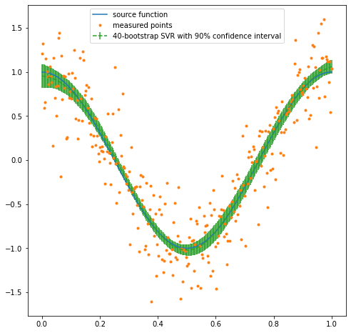
Bootstrap Uncertainty Quantification

For some cases where uncertainty intervals are necessary, resampling can be used to train multiple models, where the mean and standard deviation is then used as prediction and uncertainty. Models can even be combined in this resampling method.

from sklearn.metrics import r2_score
Train,test = train_test_split(data,test_size=0.2,shuffle=True)
models = []
for i in range(40):
    train,extra = train_test_split(Train,test_size=0.5,shuffle=True)
    svr = svm.SVR()
    svr.fit(train[features],np.ravel(train[label]))
    models.append(svr)

pred = []
std = []
for i in range(len(data)):
    predicted = []
    for j in range(len(models)):
        predicted.append(models[j].predict(data[features].values[i].reshape(-1,1)))
    pred.append(np.mean(predicted))
    std.append(1.645*np.std(predicted))

r2 = r2_score(pred,data[label])
print('ensemble r2:',r2)

plt.figure(figsize=(8,8))
plt.plot(xl,f(xl),label='source function')
plt.plot(xl,y_measured,'.',label='measured points')
plt.errorbar(xl,pred,fmt='--',label='40-bootstrap SVR with 90% prediction interval',yerr=std)
plt.legend()

ensemble r2: 0.8063013376330483

from gekko import GEKKO
m = GEKKO()
x = m.Var(0,lb=0,ub=1)
y = Bootstrap(models,m).predict(x) #function is used here
m.Obj(y)
m.solve(disp=False)
print('solution:',y.value[0])
print('x:',x.value[0])
print('Gekko Solvetime:',m.options.SOLVETIME,'s')

solution: -1.0201166145
x: 0.49964423862
Gekko Solvetime: 0.186 s

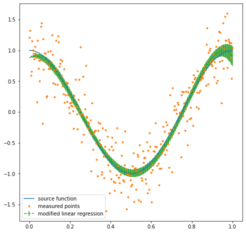
Linear Regression

Linear regression is also interfaced in Gekko. This works for Sklearn’s RidgeRegression and LinearRegression functions. For nonlinear functions, linear regression can be extended to polynomial/multivariate regression with feature engineering. It is possible to calculate the uncertainty of prediction for linear regression, so the training set and RMSE is also provided to the Interface function.

from sklearn.metrics import mean_squared_error

newdata = data
newdata['x^2'] = data['x']**2
newdata['x^3'] = data['x']**3
newdata['sinx'] = np.sin(data['x'])
newfeatures = ['x','x^2','x^3','sinx']

from sklearn.linear_model import Ridge

train,test = train_test_split(newdata,test_size=0.2,shuffle=True)

lr = Ridge(alpha=0)
lr.fit(train[newfeatures],train[label])
lr.score(test[newfeatures],test[label])
pred = lr.predict(data[newfeatures])
RMSE = np.sqrt(mean_squared_error(pred,data[label]))
Xtrain = train[newfeatures].values

#predict with the Linear model and uncertainties
import scipy.stats as ss
def predict(model,xi,Xtrain,RMSE,conf=0.9):
    pred = model.predict(xi.reshape(1,-1))[0][0]
    G = np.linalg.inv(np.dot(Xtrain.T,Xtrain))
    n = len(Xtrain)
    p = len(G)
    t = ss.t.isf(q=(1 - conf) / 2, df=n-p)
    uncertainty = RMSE*t*np.sqrt(np.dot(np.dot(xi.T,G),xi))
    return pred,uncertainty

pred = []
std = []
for i in range(len(newdata)):
    p,s = predict(lr,newdata[newfeatures].values[i],Xtrain,RMSE)
    pred.append(p)
    std.append(s)

plt.figure(figsize=(8,8))
plt.plot(xl,f(xl),label='source function')
plt.plot(xl,y_measured,'.',label='measured points')
plt.errorbar(xl,pred,fmt='--',yerr=std,label='modified linear regression')
plt.legend()

from gekko import GEKKO
m = GEKKO()
x = m.Var(.1,lb=0,ub=1)
#needs to be modified due to feature engineering
x1 = x
x2 = x**2
x3 = x**3
x4 = m.sin(x)
y = Gekko_LinearRegression(lr,m).predict([x1,x2,x3,x4]) #function is used here
m.Obj(y)
m.solve(disp=False)
print('solution:',y.value[0])
print('x:',x.value[0])
print('Gekko Solvetime:',m.options.SOLVETIME,'s')

solution: -0.99222938638
x: 0.50971895084
Gekko Solvetime: 0.013500000001 s

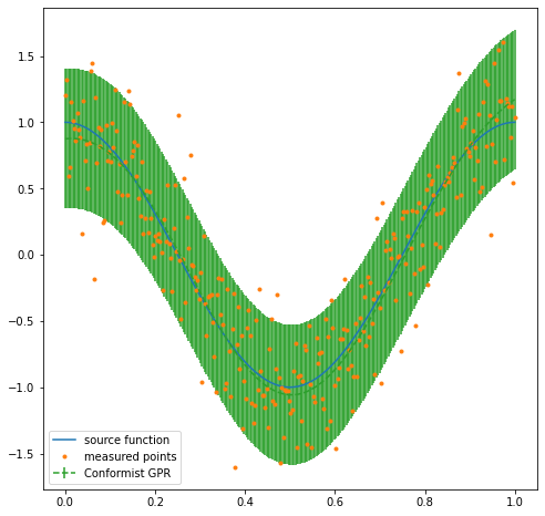
Conformal Prediction Uncertainty Quantification

Prediction intervals can also be calculated with a distance-metric based method called non-conformist prediction. This requires an additional datasplit of the training set into a training set and calibration set. This calibration set is then used to calibrate the model and give a prediction interval that represents the desired quantile. This method works with every model and produces a constant uncertainty rather than a variable one. The model is first trained with the nonconformist library before it is interfaced with Gekko. It typically results in a higher variance but can be more consistent than other methods.

from nonconformist.base import RegressorAdapter
from nonconformist.icp import IcpRegressor
from nonconformist.nc import RegressorNc, RegressorNormalizer
from nonconformist.nc import InverseProbabilityErrFunc
from nonconformist.nc import MarginErrFunc,AbsErrorErrFunc,SignErrorErrFunc
from sklearn.neural_network import MLPRegressor
import sklearn.gaussian_process as gp
from sklearn import svm

train,test = train_test_split(data,test_size=0.2,shuffle=True)
train,calibrate = train_test_split(train,test_size=0.5,shuffle=True)


k = gp.kernels.RBF() * gp.kernels.ConstantKernel() + gp.kernels.WhiteKernel()
gpr = gp.GaussianProcessRegressor(kernel=k,\
                            n_restarts_optimizer=10,\
                            alpha=0.1,\
                            normalize_y=True)


mod = RegressorAdapter(gpr)

nc = RegressorNc(mod,AbsErrorErrFunc()) #assign an error function
icp = IcpRegressor(nc) #create the icp regressor
icp.fit(train[features],train[label].values.reshape(len(train)))
icp.calibrate(calibrate[features],calibrate[label].values.reshape(len(calibrate)))

all_prediction = icp.predict(data[features].values,significance=0.1)
pred = (all_prediction[:,0] + all_prediction[:,1])/2
margin = (abs(all_prediction[:,0] - all_prediction[:,1])/2)[0]
r2a = r2_score(pred,data[label])
print('r2:',r2a)
print('90% prediction margin:',margin)

r2: 0.8134537732195808
90% prediction margin: 0.527352056347252

plt.figure(figsize=(8,8))
plt.plot(xl,f(xl),label='source function')
plt.plot(xl,y_measured,'.',label='measured points')
plt.errorbar(xl,pred,fmt='--',yerr=margin,label='Conformist GPR')
plt.legend()

from gekko import GEKKO
m = GEKKO()
x = m.Var(.1,lb=0,ub=1)
#needs to be modified due to feature engineering
y = Conformist([icp.get_params()['nc_function__model'].get_params()['model'],margin],m).predict([x])
m.Obj(y)
m.solve(disp=False)
print('solution:',y.value[0])
print('x:',x.value[0])
print('Gekko Solvetime:',m.options.SOLVETIME,'s')

solution: -0.95151964117
x: 0.51036497097
Gekko Solvetime: 0.023100000006 s

There are several methods of calculating prediction uncertainty for the interfaced models. Uncertainty is calculated within Gaussian Processes. Several models can be trained and used with resampling for a prediction mean and variation. Linear regression can create uncertainty through least squared equations. This same uncertainty method can be applied to other nonlinear regression methods with the Delta function. The nonconformist library can generate an uncertainty margin as well. Different variants of neural networks, specifically in Tensorflow, can produce uncertainty based on the loss function.

Control Applications

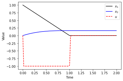
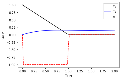
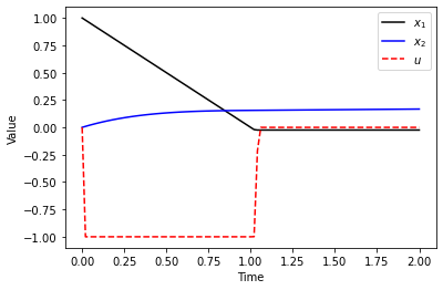
These models can be used for a wide variety of applications in Gekko, not just optimization. Here, a simple control problem is presented where the xt function is replaced by a model. It generates nearly the same result

def control1(model=[],returns=False,plot=True):
    global m

    m = GEKKO() # initialize gekko
    nt = 101
    m.time = np.linspace(0,2,nt)
    # Variables
    x1 = m.Var(value=1)
    x2 = m.Var(value=0)
    u = m.Var(value=0,lb=-1,ub=1)
    p = np.ones(nt) # mark final time point
    p[-1] = 1.0
    final = m.Param(value=p)
    # Equations
    m.Equation(x1.dt()==u)
    if(model == []):
        f = 0.5*x1**2
    else:
        if(model[0] == 'GPR'):
            f = Gekko_GPR(model[1],m).predict([x1])
        elif(model[0] == 'SVR'):
            f = Gekko_SVR(model[1],m).predict([x1])
        elif(model[0] == 'NNSK'):
            f = Gekko_NN_SKlearn(model[1],model[2],m).predict([x1])
        elif(model[0] == 'NNTF'):
            f = Gekko_NN_TF(model[1],model[2],m,1).predict([x1])

    m.Equation(x2.dt()==f)
    m.Obj(x2*final) # Objective function
    m.options.IMODE = 6 # optimal control mode
    m.solve(disp=False) # solve

    if plot:
        plt.figure(1) # plot results
        plt.plot(m.time,x1.value,'k-',label=r'$x_1$')
        plt.plot(m.time,x2.value,'b-',label=r'$x_2$')
        plt.plot(m.time,u.value,'r--',label=r'$u$')
        plt.legend(loc='best')
        plt.xlabel('Time')
        plt.ylabel('Value')
        plt.show()
    if returns:
        return m.time,x1.value,x2.value,u.value

#Generate Training set
import numpy as np
import matplotlib.pyplot as plt

def f(x):
    return 0.5*x**2

N = 200
xl = np.linspace(-2,2,N)
noise = np.random.normal(0,.1,N)
y_measured = f(xl) + noise

plt.plot(xl,f(xl),label='source function')
plt.plot(xl,y_measured,'.',label='measured points')

import pandas as pd
from sklearn.model_selection import train_test_split

data = pd.DataFrame(np.array([xl,y_measured]).T,columns=['x','y'])
features = ['x']
label = ['y']

train,test = train_test_split(data,test_size=0.2,shuffle=True)

import sklearn.gaussian_process as gp
from sklearn.neural_network import MLPRegressor
from sklearn import svm

#gpr
k = gp.kernels.RBF() * gp.kernels.ConstantKernel() + gp.kernels.WhiteKernel()
gpr = gp.GaussianProcessRegressor(kernel=k,\
                            n_restarts_optimizer=10,\
                            alpha=0.1,\
                            normalize_y=True)
gpr.fit(train[features],train[label])
r2 = gpr.score(test[features],test[label])
print('gpr r2:',r2)


#svr
svr = svm.SVR()
svr.fit(train[features],np.ravel(train[label]))
r2 = svr.score(test[features],np.ravel(test[label]))
print('svr r2:',r2)

gpr r2: 0.9786408113248649
svr r2: 0.9731400906454939

control1()

control1(["GPR",gpr])

control1(["SVR",svr])

Remarks

All of these functions import trained models and tools provided by other packages. The packages used for this extension to Gekko are:

Scikit-learn: https://scikit-learn.org/stable/

Tensorflow: https://www.tensorflow.org/

GPflow: https://github.com/GPflow/GPflow

Nonconformist: https://github.com/donlnz/nonconformist

as well as other standard packages like Numpy, Pandas, and others.

Authors of the Machine Learning package for Gekko are graduate research assistants LaGrande Gunnell and Kyle Manwaring. Thanks to John Vienna and Xiaonan Lu of Pacific Northwest National Laboratory for providing technical direction and sponsorship of the work through a Department of Energy (DOE) grant.